From Softmax to ArcFace: Building Better Embeddings with Additive Angular Margins

Introduction

Imagine trying to build a face identification system that can recognize any face on Earth, not just some fixed set of faces. New faces appear every day, and there’s no way to include all of them during training. Traditional classification methods start to fall apart in this kind of open-ended problem.

One of the most common such methods is softmax. It works brilliantly when the set of classes is fixed, but struggles when new, unseen classes appear. In this post, we’ll explore how softmax works, why it falters in open-ended scenarios, and how ArcFace, ArcFace: Additive Angular Margin Loss for Deep Face Recognition (Deng et al., 2022), addresses the problem with an additive angular margin loss that forces better separation between classes.

To keep things easy to visualize, we’ll use the first five classes of MNIST, a dataset of handwritten digits. MNIST doesn’t require ArcFace, as the classes are fixed at 10, but it’s a convenient playground for illustrating the concepts. We’ll walk through code snippets, mathematical details, and visualizations from trained models. The full source code will be available here.

A Softmax Model for MNIST

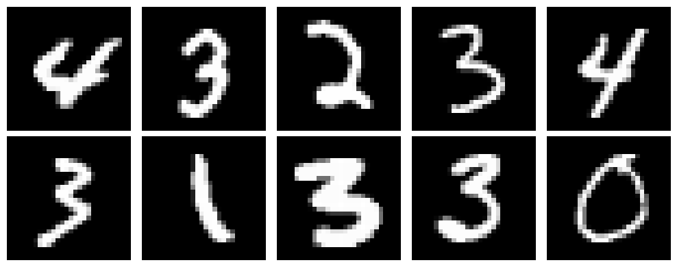
MNIST consists of 28×28 grayscale images of handwritten digits (0–9) with labels. For demonstration purposes, we will use the first 5 digits. They look like this:

At a high level, our pipeline is:

image → embedding network → classifier → probability distribution

The embedding network encodes relevant structure in an image into a vector. The classifier maps embeddings to class scores. Here’s a simple embedding network that outputs 2‑dimensional embeddings (handy for plotting):

class SimpleEmbeddingNetwork(nn.Module):
    def __init__(self, embedding_dim=2):
        super().__init__()
        self.relu = nn.ReLU()
        self.conv1 = nn.Conv2d(1, 32, kernel_size=3, padding=1, bias=False)
        self.bn1 = nn.BatchNorm2d(32)
        self.pool = nn.MaxPool2d(2, 2)
        self.conv2 = nn.Conv2d(32, 64, kernel_size=3, padding=1, bias=False)
        self.bn2 = nn.BatchNorm2d(64)
        self.fc1 = nn.Linear(64 * 7 * 7, 128, bias=False)
        self.bn3 = nn.BatchNorm1d(128)
        self.fc2 = nn.Linear(128, embedding_dim)

    def forward(self, x):
        # First convolutional block with BatchNorm
        x = self.conv1(x)
        x = self.bn1(x)
        x = self.relu(x)
        x = self.pool(x)

        # Second convolutional block with BatchNorm
        x = self.conv2(x)
        x = self.bn2(x)
        x = self.relu(x)
        x = self.pool(x)

        # Flatten the spatial dimensions
        x = x.view(-1, 64 * 7 * 7)

        # First fully connected layer with BatchNorm
        x = self.fc1(x)
        x = self.bn3(x)
        x = self.relu(x)

        # Output embedding layer
        embedding = self.fc2(x)

        return embedding

A standard softmax classifier first produces logits with a linear layer. The softmax operation is then applied, typically within the loss function during training, to convert these logits into a probability distribution:

class LinearClassifier(nn.Module):
    def __init__(self, embedding_dim=2, num_classes=5, bias=False):
        super().__init__()
        self.fc = nn.Linear(embedding_dim, num_classes, bias=bias)

    def forward(self, x):
        # Project embeddings to class logits
        logits = self.fc(x)
        return logits

Understanding this linear layer is key to understanding ArcFace. Assuming no bias, the logits are:

\[\mathbf{z} = \mathbf{x} \cdot \mathbf{W}^\top \, ,\]

where:

• $\mathbf{x}$ is the batch of embeddings (shape: batch_size × embedding_dim)
• $\mathbf{W}$ is the weight matrix (shape: num_classes × embedding_dim)

With 5 classes (digits 0–4) and an embedding size of 2, $\mathbf{W}$ has shape (5, 2). After training this simple embedding network and classifier, I ended up with:

\[\mathbf{W}^\top = \begin{bmatrix} 0.96 & -0.67 & 0.31 & 0.45 & -0.66 \\ 0.37 & -0.33 & 1.03 & -0.77 & 0.59 \\ \end{bmatrix}\]

Each column of $\mathbf{W}^\top$ (or each row of $\mathbf{W}$) is a vector $\mathbf{w}_i$ representing the class center of class $i$:

\[\begin{align*} \mathbf{w}_0 = & \begin{bmatrix} 0.96 \\ 0.37 \\ \end{bmatrix} & \mathbf{w}_1 = & \begin{bmatrix} -0.67 \\ -0.33 \\ \end{bmatrix} & \mathbf{w}_2 = & \begin{bmatrix} 0.31 \\ 1.03 \\ \end{bmatrix} \\ \mathbf{w}_3 = & \begin{bmatrix} 0.45 \\ -0.77 \\ \end{bmatrix} & \mathbf{w}_4 = & \begin{bmatrix} -0.66 \\ 0.59 \\ \end{bmatrix} \\ \end{align*}\]

We can write:

\[\mathbf{W}^\top = \begin{bmatrix} \mathbf{w}_0 & \mathbf{w}_1 & \mathbf{w}_2 & \mathbf{w}_3 & \mathbf{w}_4 \end{bmatrix}\]

Similarly, $\mathbf{x}$ is a stack of embedding row vectors:

\[\mathbf{x} = \begin{bmatrix} \mathbf{x}_0 \\ \mathbf{x}_1 \\ \mathbf{x}_2 \\ \vdots \\ \end{bmatrix}\]

We can write:

\[\mathbf{z} = \mathbf{x} \cdot \mathbf{W}^\top = \begin{bmatrix} \mathbf{x}_0 \\ \mathbf{x}_1 \\ \mathbf{x}_2 \\ \vdots \\ \end{bmatrix} \cdot \begin{bmatrix} \mathbf{w}_0 & \mathbf{w}_1 & \mathbf{w}_2 & \mathbf{w}_3 & \mathbf{w}_4 \end{bmatrix}\]

A useful way to think of the dot product of two matrices is that you are taking the dot products of the row vectors on the left with the column vectors on the right, which gives us:

\[\mathbf{z} = \begin{bmatrix} \mathbf{x}_0 \cdot \mathbf{w}_0 & \mathbf{x}_0 \cdot \mathbf{w}_1 & \mathbf{x}_0 \cdot \mathbf{w}_2 & \mathbf{x}_0 \cdot \mathbf{w}_3 & \mathbf{x}_0 \cdot \mathbf{w}_4 \\ \mathbf{x}_1 \cdot \mathbf{w}_0 & \mathbf{x}_1 \cdot \mathbf{w}_1 & \mathbf{x}_1 \cdot \mathbf{w}_2 & \mathbf{x}_1 \cdot \mathbf{w}_3 & \mathbf{x}_1 \cdot \mathbf{w}_4 \\ \mathbf{x}_2 \cdot \mathbf{w}_0 & \mathbf{x}_2 \cdot \mathbf{w}_1 & \mathbf{x}_2 \cdot \mathbf{w}_2 & \mathbf{x}_2 \cdot \mathbf{w}_3 & \mathbf{x}_2 \cdot \mathbf{w}_4 \\ \vdots & \vdots & \vdots & \vdots & \vdots \end{bmatrix}\]

So the output of the linear layer is the dot product of each embedding with each class center. These are called the logits. For each embedding, the largest logit determines the predicted class.

Embeddings and Class Centers

Each embedding produced by our network is just a point in the same space as the class center vectors. If the network has learned well, embeddings for the same class will tend to cluster in relation to their corresponding class center.

Below (left) is a scatter plot of all embeddings from the test set, colored by their true class, with the learned class centers shown as black stars. The class centers have much smaller magnitudes than the embeddings, so they appear bunched up near the origin. To make them visible, the right plot shows a zoomed-in view around the origin:

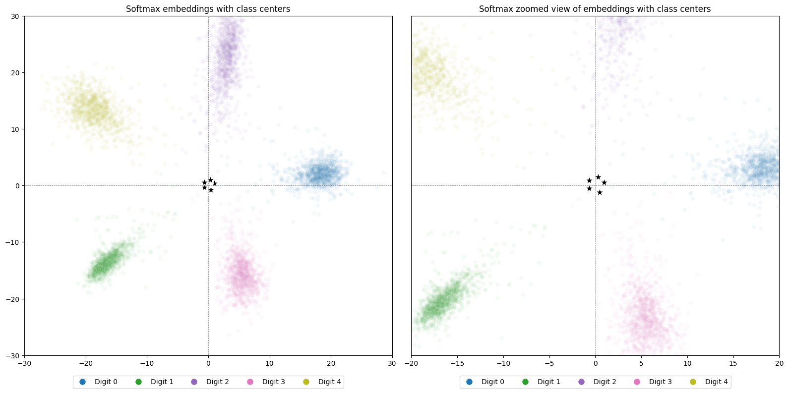
Notice how, even though the embeddings themselves are far from the origin, the class centers occupy a very small region. This scale difference is one reason we’ll later discuss normalization—to bring embeddings and class centers onto a comparable scale.

Decision Boundaries

The class center vectors also define the decision boundaries between classes. A point lies on the decision boundary between two classes when the model is equally confident in both: meaning their logits are exactly the same. In other words, the dot product of the embedding with each class center produces the same score. For any two classes $i$ and $j$, the decision boundary is the set of points where:

\[\mathbf{x} \cdot \mathbf{w}_i = \mathbf{x} \cdot \mathbf{w}_j\]

which simplifies to:

\[\mathbf{x} \cdot (\mathbf{w}_i - \mathbf{w}_j) = 0\]

This is the equation of a hyperplane passing through the origin in the embedding space. On one side of the hyperplane, class $i$ has the larger logit; on the other side, class $j$ does.

In two dimensions, these hyperplanes are simply straight lines through the origin. Here are two examples:

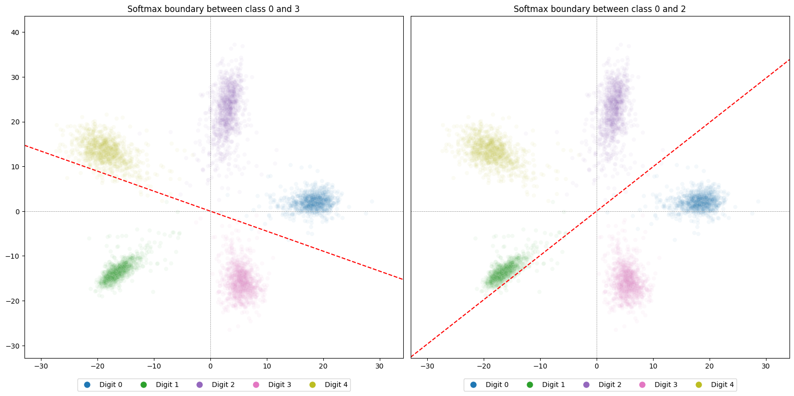
In each plot, the line marks where the logits for the two classes are equal. Points on one side give a higher logit to one class; points on the other side give a higher logit to the other. In a multi-class setting, the final predicted class is whichever has the largest logit among all classes, so a point might fall on one side of this boundary but still be predicted as some completely different class whose logit is even higher.

A Single Example

Let’s zoom in on a single example. Suppose we have an input like the following:

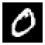
If we feed this image into our embedding network, we get the following embedding:

\[x_0 = \begin{bmatrix} 18.14 & 2.41 \\ \end{bmatrix}\]

We can write the logits, given the embedding, as:

\[\begin{align*} \mathbf{z} & = \mathbf{x} \cdot \mathbf{W}^\top \\ & = \begin{bmatrix} \mathbf{x}_0 \\ \end{bmatrix} \cdot \begin{bmatrix} \mathbf{w}_0 & \mathbf{w}_1 & \mathbf{w}_2 & \mathbf{w}_3 & \mathbf{w}_4 \end{bmatrix} \\ & =\begin{bmatrix} \mathbf{x}_0 \cdot \mathbf{w}_0 & \mathbf{x}_0 \cdot \mathbf{w}_1 & \mathbf{x}_0 \cdot \mathbf{w}_2 & \mathbf{x}_0 \cdot \mathbf{w}_3 & \mathbf{x}_0 \cdot \mathbf{w}_4 \\ \end{bmatrix} \\ & = \begin{bmatrix} \begin{bmatrix} 18.14 & 2.41 \\ \end{bmatrix} \cdot \begin{bmatrix} 0.96 \\ 0.37 \\ \end{bmatrix} & \dots & \begin{bmatrix} 18.14 & 2.41 \\ \end{bmatrix} \cdot \begin{bmatrix} -0.66 \\ 0.59 \\ \end{bmatrix} \end{bmatrix} \\ & = \begin{bmatrix} 18.30 & -13.03 & 8.16 & 6.22 & -10.52 \\ \end{bmatrix} \end{align*}\]

Here, $\mathbf{x}_0 \cdot \mathbf{w}_0$ is largest, correctly predicting the “0” class.

The dot product has a relevant geometric interpretation. It is the magnitude of the vectors scaled by the cosine of the angle between them:

\[\mathbf{v} \cdot \mathbf{u} = \|\mathbf{u}\|\|\mathbf{v}\|\cos(\theta)\]

• $\theta$ = 0°, dot product is the product of magnitudes (max positive)
• $\theta$ = 90°, dot product is 0 since $\cos(90°) = 0$
• $\theta$ = 180°, dot product is the product of magnitudes times -1 since $\cos(180°) = -1$ (max negative)

Plotting the embedding and class centers:

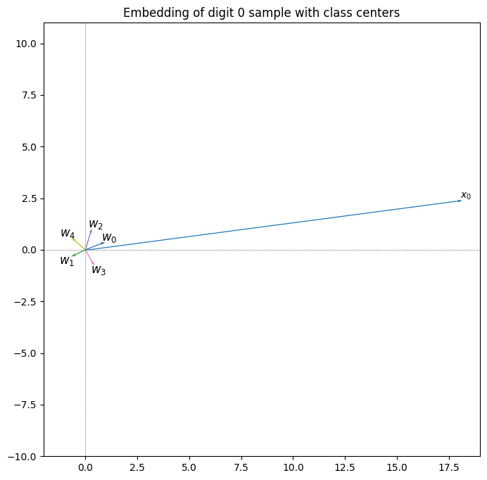
The class centers are clustered around the origin with small, similar magnitudes. $\mathbf{w}_1$ and $\mathbf{w}_4$ point roughly opposite our sample, matching their large negative dot products of -13.03 and -10.52 respectively. $\mathbf{w}_0$, $\mathbf{w}_2$, and $\mathbf{w}_3$ have angles under 90° with our sample, so their dot products are positive. Class 0’s vector, $\mathbf{w}_0$, is most aligned with the sample, giving the largest dot product: 18.30.

Softmax

Now that we’ve looked at embeddings and their relationship to the class centers, we need to figure out how to turn our logits into a probability distribution. If we look at the logits from our previous example:

\[\mathbf{z} = \begin{bmatrix} 18.30 & -13.03 & 8.16 & 6.22 & -10.52 \\ \end{bmatrix}\]

It’s clear that class 0 has the largest logit and class 1 the smallest. But logits aren’t probabilities; they can be negative, and they don’t sum to 1.

What if we transform each logit into a positive number that preserves their ordering? One way to do that is to raise a positive base to each logit. For illustration, let’s use 10 as the base:

\[\begin{aligned} 10^{18.30} & = 2.00 \times 10^{18} \\ 10^{8.16} & = 1.45 \times 10^8 \\ 10^{6.22} & = 1.67 \times 10^6 \\ 10^{-10.52} & = 3.05 \times 10^{-11} \\ 10^{-13.03} & = 9.23 \times 10^{-14} \\ \end{aligned}\]

This transformation preserves the ranking of the logits but makes all values positive. Now we can sum them and divide each by the sum to get something that behaves like a probability:

\[\begin{aligned} prob_i &= \frac{10^{z_i}}{\sum{10^{z_k}}} \\ \end{aligned}\]

In practice, softmax does the same thing, except it uses $e$ (Euler’s number) instead of 10:

\[\begin{aligned} \operatorname{softmax}(z)_i &= \frac{e^{z_i}}{\sum{e^{z_k}}} \\ \end{aligned}\]

For our example:

\[\sum{e^{z_k}} = e^{18.30} + e^{-13.03} + e^{8.16} + e^{6.22} + e^{-10.52} \\ \approx 8.85 \times 10^7\] \[\operatorname{softmax}(z) \approx \begin{bmatrix} 1.00 \\ 0.00 \\ 0.00 \\ 0.00 \\ 0.00 \\ \end{bmatrix}\]

So the model assigns essentially 100% probability to class “0” for this sample.

(In real code, we subtract $max(z)$ from all logits before exponentiating to avoid overflow issues, but the math is the same.)

Okay, now we’ve covered how to get from embeddings to a probability distribution. Next, we’ll look at why this isn’t good enough when we don’t know all the classes up front.

Trouble with Open-Ended Classes

When we have open-ended classes, like in face identification, we often need to compare two samples to decide if they belong to the same class. For example, we might compare two face images to see if they show the same person.

A softmax classifier can only recognize classes it saw during training, so for new identities it’s not reliable. Instead, we have to compare embeddings directly. If our embedding network maps members of the same class close together in embedding space, then we can decide “same class” or “different class” based on their distance.

But if we train an embedding network with a softmax classifier, do we actually get embeddings that work well for this?

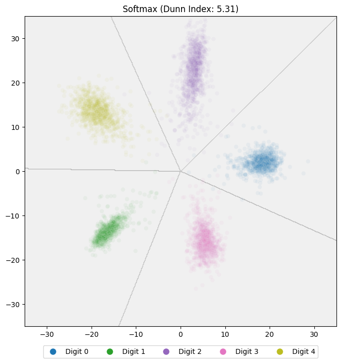
Returning to our example softmax model, here’s how it maps our test data into the embedding space:

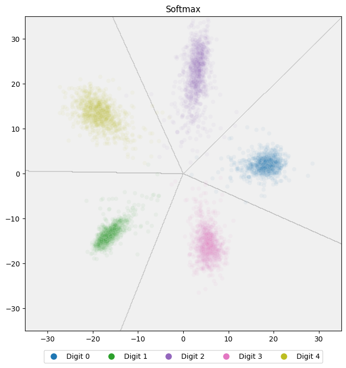
The points form loose clusters by class, and the grey lines show the classifier’s decision boundaries. Ideally, these clusters should be far apart from each other and tightly packed within each class. That way, any two points from the same class are closer to each other than to any point from another class.

But is that what we see here? Consider these samples:

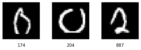
All three are classified correctly: samples 174 and 204 belong to class 0, and sample 887 belongs to class 2. However, sample 174 is closer to sample 887 than 204, both in Euclidean and cosine distance.

This means there’s no single distance threshold that would let us correctly say “174 and 204 are the same class” while “174 and 887 are different classes.” The reliability of distances in embedding space depends on both:

• Inter-class separation: how far apart the clusters are
• Intra-class compactness: how tight each cluster is

To improve our model, we need a way to quantify these properties and compare them across models. This brings us to the Dunn Index.

Dunn Index

When looking at the quality of clustering, we care about two things: how well separated the clusters are (inter-class distance) and how cohesive the classes are (intra-class distance). We want to maximize the inter-class distances and minimize the intra-class distances. The Dunn Index, A Fuzzy Relative of the ISODATA Process and Its Use in Detecting Compact Well-Separated Clusters (Dunn, J. C., 1973), is a metric for comparing these qualities. The metric has roughly the following form:

\[DI = \frac{\text{min class distance}}{\text{max distance between members of the same class}}\]

A higher value for the Dunn Index means the classes are well separated and cohesive, and a lower value means the classes are not well separated or cohesive. If we look at the above definition, there are two ways we can improve the Dunn Index:

1. Push the classes further apart, increasing the numerator.
2. Pack the members of each class closer together, decreasing the denominator.

One downside of the Dunn Index is that because it compares a minimum with a maximum, it is sensitive to outliers. As such, there are a number of variations that try to mitigate this. The one we will use here involves dropping all members of a class that are beyond the 95th percentile of the distances from the centroid of that class. This ensures that a single errant embedding does not torpedo the metric. It’s a simple way to make the Dunn Index more robust to outliers, and it works well in practice. The code for this is available in the source code repository.

If we compute the Dunn Index for our current softmax model, we get a value of 5.31. Now let’s look at how we can improve the model.

Normalized Softmax

Recall that we calculate the logits as:

\[\mathbf{z} = \begin{bmatrix} \mathbf{x}_0 \cdot \mathbf{w}_0 & \mathbf{x}_0 \cdot \mathbf{w}_1 & \mathbf{x}_0 \cdot \mathbf{w}_2 & \mathbf{x}_0 \cdot \mathbf{w}_3 & \mathbf{x}_0 \cdot \mathbf{w}_4 \\ \vdots & \vdots & \vdots & \vdots & \vdots \end{bmatrix}\]

During training, the model tries to maximize the dot product of the embeddings with the class centers for the correct class, while minimizing the dot products with all other classes. The dot product is defined as:

\[\mathbf{u} \cdot \mathbf{v} = \|\mathbf{u}\|\|\mathbf{v}\| \cos (\theta)\]

This means the model can increase the dot product in two ways:

1. Increasing the magnitudes of $\lVert \mathbf{u} \rVert$ or $\lVert \mathbf{v} \rVert$
2. Decreasing the angle $\theta$ between them

If we look at the embedding space for the standard softmax model from earlier, we see that the model turns that first ‘knob’, increasing the magnitude of the embeddings, quite a bit:

Notice how the points for each class radiate outward from the origin. This magnitude inflation has two downsides:

1. Euclidean distances between members of the same class become larger and more varied, making distance-based comparison less reliable.
2. Because the model can improve logits just by increasing magnitude, it has less incentive to minimize the angle between embeddings and class centers, so cosine distances suffer as well.

In NormFace: L₂ Hypersphere Embedding for Face Verification (Wang et al, 2017), the authors address this by normalizing both the embeddings and the class centers before computing the dot product. This forces:

\[\|\mathbf{x}_i\| = 1 \quad \text{and} \quad \|\mathbf{w}_j\| = 1\]

So the dot product is simply:

\[\mathbf{x}_i \cdot \mathbf{w}_j = \cos(\theta)\]

The logits then become:

\[\mathbf{z} = \begin{bmatrix} \frac{\mathbf{x}_0}{\lVert \mathbf{x}_0 \rVert} \cdot \frac{\mathbf{w}_0}{\lVert \mathbf{w}_0 \rVert} & \frac{\mathbf{x}_0}{\lVert \mathbf{x}_0 \rVert} \cdot \frac{\mathbf{w}_1}{\lVert \mathbf{w}_1 \rVert} & \dots & \frac{\mathbf{x}_0}{\lVert \mathbf{x}_0 \rVert} \cdot \frac{\mathbf{w}_4}{\lVert \mathbf{w}_4 \rVert} \\ \vdots & \vdots & & \vdots \end{bmatrix}\]

By removing the magnitude “shortcut,” the model must minimize angles to improve classification, which directly benefits cosine distances.

To normalize the embeddings, we modify our network’s forward(...) method:

class EmbeddingNetwork(nn.Module):
    
    # ... other methods ...

    def forward(self, x):
        # ... layers before the embedding layer ...

        # Output embedding layer
        embedding = self.fc2(x)

        # Normalize the embedding
        embedding = F.normalize(embedding, p=2, dim=1)

        return embedding

We also create a classifier that normalizes the class centers before computing the logits:

class CosineClassifier(nn.Linear):
    def __init__(self, embed_dim, num_classes, bias=False):
        super().__init__(embed_dim, num_classes, bias=bias)

    def forward(self, z):
        # Compute cosine similarity by using normalized weight vectors
        x = F.linear(z, F.normalize(self.weight, dim=1), self.bias)
        return x

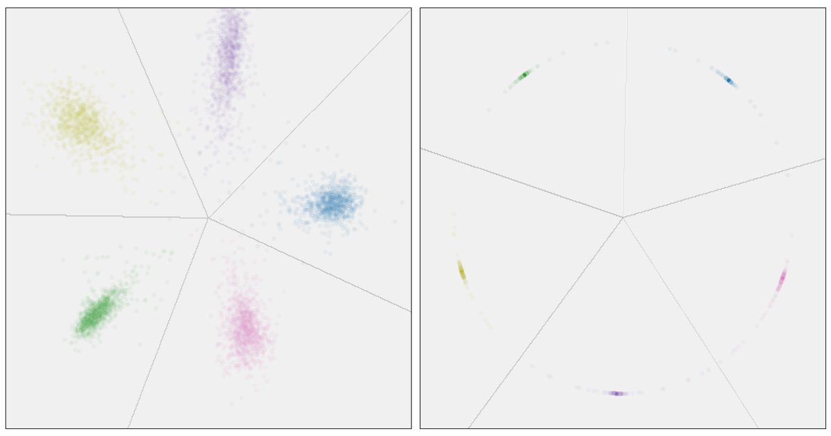
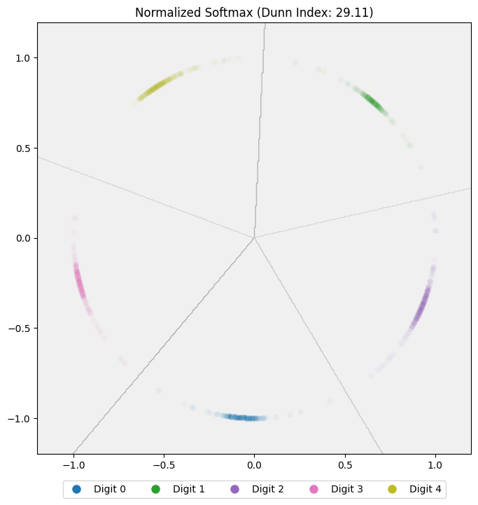
After training the normalized softmax model, the test set embeddings look like this:

Revisiting the earlier problem, where sample 174 (class 0) was closer to a sample from digit 2 than to another sample from digit 0:

We now find:

• Cosine distance between 174 and 204 (both digit 0): $2.61 \times 10^{-4}$
• Cosine distance between 174 and 887 (digit 2): $0.32$

At least for this particular case, the issue is gone: sample 174 is now embedded close to its own class and far from the other.

Calculating the Dunn Index for this normalized softmax model, we get 29.11, a clear improvement over the previous model. But we can do even better.

ArcFace Additive Margin Loss

Now that we have normalized the embeddings and class centers, rather than writing the dot product for the logits as:

\[\mathbf{z} = \begin{bmatrix} \frac{\mathbf{x}_0}{\lVert \mathbf{x}_0 \rVert} \cdot \frac{\mathbf{w}_0}{\lVert \mathbf{w}_0 \rVert} & \frac{\mathbf{x}_0}{\lVert \mathbf{x}_0 \rVert} \cdot \frac{\mathbf{w}_1}{\lVert \mathbf{w}_1 \rVert} & \dots & \frac{\mathbf{x}_0}{\lVert \mathbf{x}_0 \rVert} \cdot \frac{\mathbf{w}_4}{\lVert \mathbf{w}_4 \rVert} \\ \vdots & \vdots & & \vdots \end{bmatrix}\]

We can instead write it as:

\[\mathbf{z} = \begin{bmatrix} \cos(\theta_{\mathbf{x}_0,\mathbf{w}_0}) & \cos(\theta_{\mathbf{x}_0,\mathbf{w}_1}) & \dots & \cos(\theta_{\mathbf{x}_0,\mathbf{w}_4}) \\ \vdots & \vdots & & \vdots \end{bmatrix}\]

Here, $\theta_{\mathbf{x}_0,\mathbf{w}_i}$ is the angle between the embedding $\mathbf{x}_0$ and the class center $\mathbf{w}_i$. We can do this because the dot product is $\lVert u \rVert \lVert v \rVert \cos(\theta)$, and after normalization the magnitudes are both 1, so the dot product is simply the cosine of the angle.

Where ArcFace comes in is by adding an angular margin to the correct class during training. If $m$ is the margin (a hyperparameter), then for a sample $\mathbf{x}_0$ of class 0 the logits become:

\[\mathbf{z} = \begin{bmatrix} \cos(\theta_{\mathbf{x}_0,\mathbf{w}_0} + m) & \cos(\theta_{\mathbf{x}_0,\mathbf{w}_1}) & \dots & \cos(\theta_{\mathbf{x}_0,\mathbf{w}_4}) \\ \vdots & \vdots & & \vdots \end{bmatrix}\]

What does this do? Suppose $\theta_{\mathbf{x}_0,\mathbf{w}_i}$ is 0.5 radians (~29°). Then the original logit is $\cos(0.5) \approx 0.88$. With $m=0.5$, it becomes:

\[\cos(\theta_{\mathbf{x}_0,\mathbf{w}_0} + m) = \cos(0.5 + 0.5) \approx 0.54\]

This effectively reduces the probability of the sample being classified as the correct class and increases the probability of it being classified as one of the other classes. During training, this forces the model to reduce the angles, $\theta$, even further between the embeddings and the class centers. By reducing the angles, we pull samples away from the class boundaries and towards the class centers, which creates more cohesive clusters and better separates the classes.

To help us understand how to implement this, let’s look at a real example. Consider the sample that we used earlier:

Since this is a different model, we will have a different embedding for the sample, which is:

\[\mathbf{x}_0 =\begin{bmatrix} 0.62 & 0.78 \\ \end{bmatrix}\]

We have the following for our classifier weights, $W^T$:

\[\mathbf{W}^\top = \begin{bmatrix} 0.37 & -0.35 & -0.05 & 0.34 & -0.45 \\ 0.46 & 0.49 & -1.19 & -0.12 & -0.14 \\ \end{bmatrix}\]

Which gives us the following class centers:

\[\begin{align*} \mathbf{w}_0 = & \begin{bmatrix} 0.37 \\ 0.46 \\ \end{bmatrix} & \mathbf{w}_1 = & \begin{bmatrix} -0.35 \\ 0.49 \\ \end{bmatrix} & \mathbf{w}_2 = & \begin{bmatrix} -0.05 \\ -1.19 \\ \end{bmatrix} \\ \mathbf{w}_3 = & \begin{bmatrix} 0.34 \\ -0.12 \\ \end{bmatrix} & \mathbf{w}_4 = & \begin{bmatrix} -0.45 \\ -0.14 \\ \end{bmatrix} \end{align*}\]

The logits are computed as follows:

\[\begin{align*} \mathbf{z} & = \begin{bmatrix} \mathbf{x}_0 \cdot \mathbf{w}_0 & \mathbf{x}_0 \cdot \mathbf{w}_1 & \mathbf{x}_0 \cdot \mathbf{w}_2 & \mathbf{x}_0 \cdot \mathbf{w}_3 & \mathbf{x}_0 \cdot \mathbf{w}_4 \\ \end{bmatrix} \\ & = \begin{bmatrix} \begin{bmatrix} 0.62 & 0.78 \\ \end{bmatrix} \cdot \begin{bmatrix} 0.37 \\ 0.46 \\ \end{bmatrix} & \dots & \begin{bmatrix} 0.62 & 0.78 \\ \end{bmatrix} \cdot \begin{bmatrix} -0.45 \\ -0.14 \\ \end{bmatrix} \end{bmatrix} \\ & = \begin{bmatrix} 0.59 & 0.16 & -0.96 & 0.11 & -0.39 \\ \end{bmatrix} \\ & = \begin{bmatrix} \cos(\theta_{\mathbf{x}_0,\mathbf{w}_0}) & \dots & \cos(\theta_{\mathbf{x}_0,\mathbf{w}_4}) \\ \end{bmatrix} \end{align*}\]

We have the logits, and consequently the angles, \(\theta\), between the embedding and the class centers. We get all of this already from the normalized softmax model. Now we just need to add the margin, $m$, to the angle for the correct class. Let’s say we choose a margin of 0.5 radians. The correct class is 0, so we need to find the value of \(\cos(\theta_{\mathbf{x}_0,\mathbf{w}_0} + m)\). Well, we know \(\cos(\theta_{\mathbf{x}_0,\mathbf{w}_0})=0.59\)… but how do we add the margin? Many years ago, back in trigonometry class, you were learning about trigonometric identities and were probably wondering when you would ever possibly use them. Well, today is the day! We can use the cosine addition formula to compute this:

\[\cos(\theta + m) = \cos(\theta)\cos(m) - \sin(\theta)\sin(m)\]

We know $\cos(\theta_{\mathbf{x}_0,\mathbf{w}_0}) = 0.59$, and we can compute $\cos(m)$ and $\sin(m)$ since we know the margin, $m$, is 0.5 radians:

\[\begin{align*} \cos(m) & = \cos(0.5) \approx 0.88 \\ \sin(m) & = \sin(0.5) \approx 0.48 \end{align*}\]

Now we just need to compute $\sin(\theta_{\mathbf{x}_0,\mathbf{w}_0})$. We can do this using the Pythagorean identity:

\[\sin^2(\theta) + \cos^2(\theta) = 1 \quad\rightarrow\quad \sin(\theta) = \sqrt{1 - \cos^2(\theta)}\]

So we have:

\[\sin(\theta_{\mathbf{x}_0,\mathbf{w}_0}) = \sqrt{1 - (\cos(\theta_{\mathbf{x}_0,\mathbf{w}_0}))^2} = \sqrt{1 - 0.59^2} \approx 0.81\]

Now we can compute the logit for the correct class:

\[\begin{align*} z_0 & = \cos(\theta_{\mathbf{x}_0,\mathbf{w}_0} + m) \\ & = \cos(\theta_{\mathbf{x}_0,\mathbf{w}_0})\cos(m) - \sin(\theta_{\mathbf{x}_0,\mathbf{w}_0})\sin(m) \\ & = 0.59 \cdot 0.88 - 0.81 \cdot 0.48 \\ & \approx 0.13 \end{align*}\]

Before we get to the code, there is one more pesky little problem. When we add this margin to a logit, the goal is to make the logit smaller so that it is harder to classify the sample correctly. However, there is an edge case where adding the margin actually increases the logit. Suppose by some twist of fate \(\theta_{\mathbf{x}_0,\mathbf{w}_0}\) is actually \(\pi\) radians. In this scenario, the \(\cos(\theta_{\mathbf{x}_0,\mathbf{w}_0})\) would be -1, the smallest possible value for the cosine of an angle. If we add a margin of 0.5 radians, then we would have \(\cos(\theta_{\mathbf{x}_0,\mathbf{w}_0} + m) = \cos(\pi + 0.5) \approx -0.88\). This is actually larger than -1, which is not what we want. This situation can occur whenever \(\theta_{\mathbf{x}_0,\mathbf{w}_0} \in (\pi - m, \pi]\), which is equivalent to \(\cos(\theta_{\mathbf{x}_0,\mathbf{w}_0}) < \cos(\pi - m)\).

So how do we fix this problem? Well, the paper doesn’t seem to address this case. If we think about the scenario when this happens, it is when the embedding is pointing in the opposite direction of the class center. If the embedding and the class center are pointing in opposite directions, then the logit for the correct class would already be quite small. Sure adding the margin might, unintentionally, increase the size of the logit instead of decreasing it, but it’s a small mercy for a very small logit. My solution to the problem is to just pretend it doesn’t exist, and it seems to work well enough in practice.

With all of that out of the way, here is the code for ArcFace Additive Margin Loss:

class ArcFaceLoss(nn.Module):
    def __init__(self, s=30.0, m=1.0):
        super().__init__()
        self.update_hyperparameters(m=m, s=s)

    def update_hyperparameters(self, s=None, m=None):
        if s is not None:
            self.s = s
        if m is not None:
            self.m = m
            # Recompute trigonometric values for the new margin
            self.cos_m = math.cos(m)
            self.sin_m = math.sin(m)

    def forward(self, cos_theta, labels):
        # Clamp cosine values to avoid numerical instability
        cos_theta = torch.clamp(cos_theta, -1.0 + 1e-7, 1.0 - 1e-7)

        # Compute sine values using the Pythagorean identity:
        #
        #   sin²(θ) + cos²(θ) = 1
        #   sin(θ) = √(1 - cos²(θ))
        #
        sin_theta = torch.sqrt(1.0 - torch.pow(cos_theta, 2))

        # Apply the angular margin penalty: cos(θ+m)
        # Using the trigonometric addition formula:
        #
        #   cos(θ+m) = cos(θ)cos(m) - sin(θ)sin(m)
        #
        phi = cos_theta * self.cos_m - sin_theta * self.sin_m

        # Create one-hot encoding of labels
        one_hot = (
            F.one_hot(labels, num_classes=cos_theta.size(1))
            .float()
            .to(cos_theta.device)
        )

        # Apply margin penalty only to the target class logits
        logits = cos_theta * (1 - one_hot) + phi * one_hot

        # Apply scaling and compute cross-entropy loss
        loss = F.cross_entropy(self.s * logits, labels)
        return loss

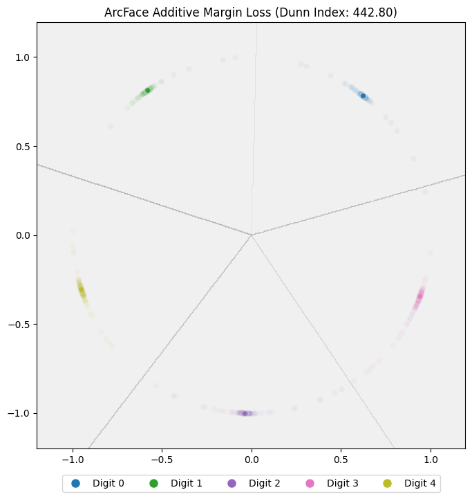
After training the model, we get a Dunn Index of 442.80, substantially better than the 29.11 we got with the normalized softmax model, and we can see this visually by looking at the embeddings for the test data:

Odds and Ends

Typically with both ArcFace and Normalized Softmax, we would use a scaling factor, $s$, to scale the logits (you can see this in the code above). The reason for this is that the logits, being cosine values, are in a very small range between -1 and 1. What this means is that our probability distribution will be very flat, with all classes having similar probabilities. For example, consider the following logits:

\[\mathbf{z} = \begin{bmatrix} 1.0 & -1.0 & -1.0 & -1.0 & -1.0 \\ \end{bmatrix}\]

For class 0, we have the highest possible logit under normalized softmax: 1.0. This is because the largest value cosine function can take is 1.0. For all the other classes, we have the lowest possible logit under normalized softmax: -1.0. If we apply the softmax function to these logits, we get:

\[\begin{align*} \operatorname{softmax}(\mathbf{z}) & = \begin{bmatrix} \frac{e^{1.0}}{\sum{e^{z_i}}} & \frac{e^{-1.0}}{\sum{e^{z_i}}} & \dots & \frac{e^{-1.0}}{\sum{e^{z_i}}}\\ \end{bmatrix} \\ & \approx \begin{bmatrix} 0.65 & 0.09 & 0.09 & 0.09 & 0.09 \end{bmatrix} \end{align*}\]

In the best possible case, the maximum probability we can assign to a class is 65%. What this can look like during training is that the model will exhibit the signs of high bias, and fail to fit the training data well. Multiplying the logits by a scaling factor, $s$, can help with this by increasing the range of values the logits can take. For example, here is what happens if we multiply the logits by a scaling factor of 20:

\[\begin{align*} \mathbf{z} & = 20 \cdot \begin{bmatrix} 1.0 & -1.0 & -1.0 & -1.0 & -1.0 \\ \end{bmatrix} \\ & = \begin{bmatrix} 20.0 & -20.0 & -20.0 & -20.0 & -20.0 \\ \end{bmatrix} \end{align*}\] \[\begin{align*} \operatorname{softmax}(\mathbf{z}) & = \begin{bmatrix} \frac{e^{20.0}}{\sum{e^{z_i}}} & \frac{e^{-20.0}}{\sum{e^{z_i}}} & \dots & \frac{e^{-20.0}}{\sum{e^{z_i}}}\\ \end{bmatrix} \\ & \approx \begin{bmatrix} 1.0 & 0.0 & 0.0 & 0.0 & 0.0 \end{bmatrix} \end{align*}\]

Now we can have probabilities effectively ranging from 0% to 100%, better enabling the model to fit the data. For the toy example we have been using, it really wasn’t necessary to use a scaling factor, but in practice it would be. The ArcFace and NormFace papers take different approaches to how the scaling factor is specified. NormFace adds a new scaling factor parameter which is learned during training while ArcFace uses a hyperparameter.

Another thing to address is that when we started I explained that we need embeddings with meaningful spatial relationships so that we can reliably handle classes not in the training data. However, so far, I’ve only shown examples for classes the model has seen during training. There are really two things we need for this to work: the embeddings need to be well clustered, and the embedding network must be able to generalize to unseen classes. The first part is what we have been focusing on here. Unfortunately, to get an embedding network that can generalize to unseen classes would take a much greater diversity of classes. Five classes representing digits is simply not enough for the embedding network to abstract the qualities that make a symbol distinct from any other symbol. For context, one of the smaller large-scale datasets you might use for training a face identification model is the VGGFace2 dataset (Cao et al., 2018) with approximately 9,000 unique identities, far more diversity than our toy dataset provides.

Conclusion

In this post, we used a toy example of classifying 5 digits (digits 0–4) from the MNIST dataset to train and compare three different models: a standard softmax model, a normalized softmax model, and an ArcFace model. We examined how well clustered the embeddings were for each model, both visually and using the Dunn Index.

We saw that the standard softmax leaves significant room for improvement in clustering quality. The normalized softmax improves clustering by normalizing the embeddings and class centers before computing the logits, forcing the model to focus on minimizing the angle between embeddings and class centers. ArcFace builds on this by adding an angular margin to the correct class during training, pulling samples farther from class boundaries and closer to their class centers.

Although our example was limited to a small set of classes, these same techniques form the foundation of state-of-the-art systems for tasks like face recognition. By understanding and applying them, you can create embedding spaces that are more discriminative, more robust, and better suited to downstream tasks that rely on meaningful spatial relationships between embeddings.